
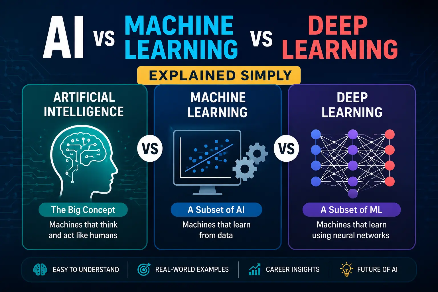
The Architectural Divide: A Deep-Dive Guide to AI, Machine Learning, and Deep Learning
For software engineers, data scientists, and computational architects, distinguishing between artificial intelligence (AI), machine learning (ML), and deep learning (DL) is not a semantic exercise. It is a foundational requirement for selecting algorithms, designing hardware pipelines, and allocating compute budgets. As deployment environments move from centralized cloud instances to local edge devices, understanding where one paradigm ends and another begins has real-world design implications.
This analysis breaks down the structural, mathematical, and physical boundaries of these three domains. We examine their optimization models, the transition from manual feature engineering to automated representation extraction, and how specialized silicon is reshaping execution.
1. The Hierarchical Taxonomy of Compute and Representation
The relationship between artificial intelligence, machine learning, and deep learning is best understood as a set of nested structures. Artificial intelligence serves as the broad outermost domain, containing any computational system designed to mimic human cognitive capabilities. Machine learning resides inside this boundary, representing the statistical methods that allow systems to improve on tasks over time using experience. At the center is deep learning, a highly specialized subset of machine learning that uses multi-layered neural networks to process raw, unstructured data.
┌────────────────────────────────────────────────────────┐
│ ARTIFICIAL INTELLIGENCE (Logic, Reason, Heuristics)    │
│ e.g., Expert Systems, Symbolic Logic, Deep Blue        │
│   ┌────────────────────────────────────────────────┐   │
│   │ MACHINE LEARNING (Statistical Representation)  │   │
│   │ e.g., Linear Regression, Random Forests, SVMs  │   │
│   │   ┌────────────────────────────────────────┐   │   │
│   │   │ DEEP LEARNING (Multi-layer Networks)   │   │   │
│   │   │ e.g., Transformers, CNNs, Autoencoders │   │   │
│   │   └────────────────────────────────────────┘   │   │
│   └────────────────────────────────────────────────┘   │
└────────────────────────────────────────────────────────┘
The Limits of Symbolic AI and Expert Systems
Early artificial intelligence relied on symbolic logic and deductive reasoning. These systems used static databases of human knowledge combined with inference engines to draw conclusions. If an engineer wanted to build a maze-navigation program or a medical triage system, they had to write every decision path by hand.
This rules-based approach reached its limit when handling dynamic, real-world variables. The computational rules of classical AI are rigid: they can execute deterministic logic but cannot learn from experience.
For example, IBM’s chess-playing computer, Deep Blue, could evaluate 200 million distinct chess board positions per second using heuristic evaluation functions. Yet, it remained a "weak" or "narrow" AI. It was incapable of generalizing its strategic knowledge or improving its play beyond its programmed rules.
The Transition to Inductive Statistical Learning
Machine learning shifts the programming paradigm from a deductive approach to an inductive one. Instead of coding rules to evaluate inputs, engineers provide a machine learning algorithm with structured data and let it mathematically determine the optimal decision boundaries.
Using statistical methods like regression, decision trees, or support vector machines (SVMs), the system builds a representative model from training data. This allows it to make predictions on unseen data points.
The system relies on structured, tabular inputs. Here, human domain experts must curate and label the data features before the learning process begins.
The Scale of Deep Representations
Deep learning scales this inductive process by using multi-layered artificial neural networks. The "deep" in deep learning refers directly to the presence of multiple hidden layers between the input and output nodes. While traditional neural networks in the late 20th century were shallow—typically featuring only two or three hidden layers—modern deep learning architectures can scale to over 150 layers.
Rather than relying on human developers to identify and format relevant features, these deep networks use backpropagation and gradient descent to automatically discover hierarchical patterns directly from raw, unstructured data.
2. Mathematical and Algorithmic Foundations
The operational differences between these paradigms are rooted in their mathematical designs. Traditional machine learning relies on linear algebra, calculus, and probability theory to optimize parameter values for relatively simple functions. Deep learning, by contrast, maps inputs to outputs through high-dimensional non-linear coordinate transformations.
Mathematical Mechanics of Traditional ML Models
Traditional machine learning algorithms are designed around clear, interpretable mathematical formulas. To illustrate:
-
Logistic Regression: Maps input values to probabilities using the sigmoid activation function:
-
Support Vector Machines (SVMs): Find the optimal separating hyperplane in high-dimensional spaces. They use the "kernel trick" to map non-linear input features into a higher-dimensional space where they become linearly separable.
-
Decision Trees: Partition feature spaces recursively based on metrics like Information Gain or Gini Impurity:
These models are mathematically straightforward to train. They can run on basic CPU hardware and require relatively few data points to reach convergence.
ALSO READ: AI API Platforms how developers are choosing their
Mathematical Mechanics of Deep Neural Networks
In contrast to traditional models, Andrew Ng notes that supervised deep learning is fundamentally a multidimensional curve-fitting procedure. Despite references to biological brains, deep learning is built on linear transformations paired with non-linear activation functions.
An individual neuron within a network layer computes a weighted sum of its inputs, adds a bias, and passes the result through an activation function like the Rectified Linear Unit (ReLU):
Where $W^{[l]}$ is the weight matrix for layer $l$, $a^{[l-1]}$ is the activation vector from the preceding layer, $b^{[l]}$ is the bias vector, and $g$ is the activation function.
Input Layer (a⁰) ──► [ W¹, b¹ ] ──► Activation g(z¹) ──► Hidden Layer (a¹) ──► [ W², b² ] ──► Output (a²)
According to circuit theory in computational mathematics, there are certain complex functions that would require an exponential number of hidden units to fit in a shallow network. By using a deep architecture, these same functions can be represented efficiently using a fraction of the nodes.
Get Extra 20% OFF
Launch your website today with ultra-fast, secure & premium hosting from Hostinger. Click to claim your deal!
Training these deep networks requires managing issues like vanishing and exploding gradients. If the network weights are initialized poorly, gradients can shrink or grow exponentially during backpropagation, causing the model to stall or fail.
To prevent this, engineers use techniques like Xavier initialization for tanh activation functions. This approach balances the variance of weight matrices across layers to maintain stable gradient flow:
Optimization at this scale also requires managing the tradeoff between mini-batch sizes. Large mini-batch sizes can slow down training iterations, while small sizes speed up processing but can lead to unstable convergence.
A common best practice is to select a balanced mini-batch size (typically between 64 and 512) that takes advantage of GPU vectorization techniques while maintaining steady convergence.
3. Feature Engineering: The Human-Machine Boundary
The division of labor between machine and engineer differs significantly between traditional machine learning and deep learning.
Traditional ML and Feature Engineering Tools
Traditional machine learning algorithms cannot easily process raw, unstructured input data. If raw audio signals or raw pixel matrices are passed directly to an SVM or a random forest, the model's accuracy will drop.
Instead, traditional ML depends on manual feature engineering. This is the process of transforming raw inputs into structured columns that expose the underlying patterns to the algorithm.
[Raw Data] ──► [Domain Expert Feature Selection] ──► [Traditional Algorithm] ──► Prediction
This manual transformation step requires significant domain expertise and iterative trial-and-error. In spatial image tasks, engineers must construct feature descriptors such as the Scale-Invariant Feature Transform (SIFT) or Histogram of Oriented Gradients (HOG).
In time-series or acoustic tasks, raw signal waveforms must be converted into numerical representations like Mel-Frequency Cepstral Coefficients (MFCCs).
To automate some of this manual work, the data science community has developed automated feature engineering libraries. These tools are highly useful for structured and relational datasets:
-
Tsfresh: A Python library that automatically extracts hundreds of statistical features from time-series datasets. It uses hypothesis testing to filter out uninformative features.
-
Featuretools: An open-source framework for automated feature engineering on relational tables. It uses Deep Feature Synthesis to generate features across linked database tables.
-
getML: A specialized tool designed for automated feature engineering on relational database architectures. It is built with a C/C++ engine to accelerate feature synthesis.
-
One-Button Machine (OneBM): An automated framework that combines feature transformation and feature selection across relational tables, helping non-experts quickly build useful representations.
Automated Representation Learning in Deep Learning
Deep learning takes a different approach by performing automated representation learning. It processes raw, unstructured data directly, bypassing the need for manual feature engineering.
[Raw Data] ──► [Deep Neural Network (Learns Features Internally)] ──► Prediction
In a Convolutional Neural Network (CNN) trained to identify objects, the early layers learn to detect simple features like edges and gradients. The middle layers combine these edges to identify more complex textures and shapes. Finally, the deepest layers assemble these shapes into recognizable object components.
This approach is highly effective for complex tasks. For example, in the unsupervised analysis of complex physical systems or bio-signals, researchers compared expert-driven feature pipelines against automated 1D-convolutional autoencoders (CAEs).
While the human-engineered feature pipeline achieved a Silhouette clustering score of 0.6441, the automated 1D-CAE matched this performance with a score of 0.6415. Crucially, the autoencoder achieved a significantly lower noise ratio (0.74% compared to 1.5% for manual engineering). This demonstrated the model's ability to extract clean features directly from complex, non-linear signals without human bias or manual pipeline design.
ALSO READ: CHAT GPT VS GEMINI VS CLUADE
4. Empirical Scaling and Data-Centric AI Strategy
The performance scaling of machine learning and deep learning models depends heavily on data volume.
The Saturation Phenomenon
Traditional machine learning algorithms benefit from small to medium-sized datasets, typically ranging from a few thousand to tens of thousands of samples. However, as the volume of training data grows, their learning curves inevitably flatten.
Past this saturation point, adding more data yields negligible accuracy improvements. The mathematical simplicity of these models prevents them from using the additional data to resolve complex, non-linear patterns.
Deep learning models, on the other hand, do not saturate as easily. Their performance continues to scale with larger datasets, provided they have the computational capacity to match.
Get Extra 20% OFF
Launch your website today with ultra-fast, secure & premium hosting from Hostinger. Click to claim your deal!
When trained on millions of labeled data points, a deep neural network will consistently outperform traditional algorithms. In small-data environments (fewer than 10,000 samples), however, traditional machine learning models often match or exceed the accuracy of deep models.
This is because deep neural networks have millions of trainable parameters, making them highly prone to overfitting when data is scarce.
Modern Labeled Splits and Data-Centric AI
This difference in data scale has reshaped the standard methodologies used in ML project workflows. In the classical era of machine learning, datasets were typically split using a 70/30 or 60/20/20 ratio for training, validation, and testing.
For modern deep learning projects with datasets in the millions, these splits have shifted to 98/1/1 or even 99/0.5/0.5. With 10 million examples, 1% of the dataset (100,000 samples) is statistically sufficient to provide clear confidence bounds during model validation.
Additionally, engineering focus is shifting from model-centric optimization (where the data is kept static while engineers iteratively adjust the neural network architecture) to Data-Centric AI. This paradigm treats the model code as fixed and focuses on iteratively improving the quality, consistency, and labeling of the training dataset.
   ┌─────────────────────────────────────────────────────────┐
   │                  THE DATA-CENTRIC AI CYCLE             │
   └────────────────────────────┬────────────────────────────┘
                                │
                                ▼
                       Train Baseline Model
                                │
                                ▼
                      Perform Error Analysis
               (Find where model fails, e.g., noisy data)
                                │
                                ▼
                  Improve and Clean Data Quality
         (Resolve ambiguous labels, collect missing samples)
                                │
                                └───────────────────────────────────────┘
This iterative cycle is highly effective. For instance, in automated speech recognition, training data often contains inconsistent or ambiguous audio labels.
Measuring labeler consistency and refining labeling guidelines allows teams to systematically improve dataset quality. This data-centric approach can yield significant accuracy improvements, often outperforming weeks of hyperparameter tuning.
This shift also influences how engineers measure and evaluate bias. In tasks like speech and image recognition, human-level error is often used as a practical proxy for Bayes error (the theoretical minimum error rate for a given problem).
Measuring the gap between human performance and model accuracy allows development teams to quantify the system's avoidable bias and prioritize their data collection efforts accordingly.
5. Governance and Explainability: White-Box vs. Black-Box
Deploying models in production requires balancing predictive accuracy with model transparency and governance.
[Internal Link: Designing Compliant AI Systems under the EU AI Act]
Performance Tradeoffs in High-Stakes Domains
In low-stakes applications like movie recommendations, black-box models are widely used. However, in high-stakes fields like cybersecurity, medical diagnostics, and credit scoring, the lack of model transparency is a significant operational challenge.
A study evaluating AI models in cybersecurity highlighted this trade-off. For complex tasks like malware classification and intrusion detection, a deep neural network (black-box) achieved 96% accuracy, while a standard decision tree (white-box) reached only 87%.
However, for simpler classification tasks with clear decision boundaries—such as phishing URL detection—the decision tree performed competitively, achieving 90% accuracy while remaining highly interpretable.
Explainable AI (XAI) Methods
To use high-accuracy deep learning models in regulated environments, organizations apply post-hoc interpretability techniques. These tools construct local approximations to explain how a black-box model reaches its predictions:
-
LIME (Local Interpretable Model-agnostic Explanations): Perturbs the features of an input sample and observes the resulting changes in the model's predictions. It uses this data to train a simple, interpretable model (like a linear regressor) to explain the local decision boundary.
-
SHAP (Shapley Additive Explanations): Computes the marginal contribution of each feature to the final prediction based on cooperative game theory. It provides a mathematically rigorous way to assign credit to each input variable.
6. The Edge AI Paradigm Shift and Silicon Architecture
The computing landscape is undergoing a significant transition, driven by the physical and economic limits of cloud-only architectures.
The Growth of the Edge Accelerator Market
Streaming high-bandwidth telemetry or multi-channel video data to a centralized cloud instance is expensive, latency-sensitive, and often challenging for data privacy compliance. This has driven the rapid growth of the edge accelerator market.
According to market research, the global edge AI hardware market is projected to grow from USD 26.14 billion in 2025 to USD 58.90 billion by 2030, representing a 17.6% CAGR. Within this space, the market for dedicated AI accelerators is growing even faster, projected to rise from USD 7.45 billion in 2025 to USD 35.75 billion by 2030 at a 31% CAGR.
NPU Architecture and Hardware Spectra
Neural Processing Units (NPUs) achieve high energy efficiency through dedicated design. In modern silicon, moving data between processors and external memory consumes significantly more energy than the actual arithmetic calculations.
NPUs solve this issue by using dedicated on-chip memory hierarchies. These structures keep model weights and activations as close to the arithmetic units as possible, minimizing external memory access and drastically reducing power consumption.
The hardware spectrum for running these localized models is broad, spanning from tiny microcontrollers to high-performance modular units:
TinyML Workloads                                                Edge Server Workloads
[ sub-50 mW Cortex-M MCUs ] ──► [ 2.5W - 15W Edge NPUs ] ──► [ 130W System Modules ]
(Simple sensory models)   (Quantized SLMs)  (Jetson Thor Dev-kits)
Get Extra 20% OFF
Launch your website today with ultra-fast, secure & premium hosting from Hostinger. Click to claim your deal!
At the high-performance end, developer kits like Nvidia's Jetson Thor deliver up to 275+ TOPS of computational power for autonomous robotics.
Small Language Models and Post-Quantum Security
These hardware developments are accompanied by the rise of Small Language Models (SLMs) and Micro LLMs. By using compression techniques like quantization (converting 32-bit floats to 8-bit or 4-bit integers), developers can shrink massive models into efficient, task-specific packages that run locally on edge hardware.
In industrial plants and retail spaces, localized SLMs run predictive maintenance algorithms and process camera-based inspection feeds directly at the point of work. This transition enables edge devices to make fast, autonomous decisions without a continuous cloud connection.
This distributed edge architecture also introduces new security challenges. Because these devices are deployed in the field, they are vulnerable to physical access and side-channel analysis.
To protect these systems, next-generation edge devices are incorporating post-quantum cryptography (PQC). Secure control hardware—such as Lattice MachXO5-NX or low-power FPGAs from the Lattice Nexus and Avant platforms—is increasingly used to secure physical interfaces, perform sensor fusion, and run small, specialized neural networks in a secure local environment.
7. Comparative Technical Framework AI vs Machine Learning vs Deep Learning
To help engineers choose the right architecture for their projects, the following matrix compares the computational, data, and execution requirements of these paradigms:
| Metric | Artificial Intelligence (AI) | Machine Learning (ML) | Deep Learning (DL) |
| Optimization Focus |
Mimicking logical reasoning and expert-defined decision trees. |
Fitting statistical models to structured, tabular datasets. |
Multi-layered non-linear feature extraction and mapping. |
| Data Requirements |
Independent of data scale; relies entirely on coded rule engines. |
Small to medium datasets (1,000 to 10,000 tabular rows). |
Massive unstructured datasets (millions of data points). |
| Feature Extraction |
Manually encoded by human developers using symbolic rules. |
Requires manual feature engineering and preprocessing. |
Learned automatically via backpropagation through hidden layers. |
| Computational Hardware |
Low power; runs on standard CPUs. |
Moderate power; training is easily handled by standard CPUs. |
Very high power; requires parallel accelerators like GPUs or NPUs. |
| Explainability |
High; decision logic is traceable and rule-based. |
High to moderate; white-box models are directly auditable. |
Low; opaque black-box models require post-hoc interpretability. |
9. Conclusion
Deciding whether to deploy a traditional machine learning model or a deep neural network depends on the specific constraints of the project. Traditional machine learning models remain highly effective for structured, tabular datasets. They are resource-efficient, require relatively little data, and provide the transparency needed for regulated industries.
Deep learning models are highly useful for processing unstructured data like raw images, speech, and text. However, this capabilities-first approach requires substantial computational infrastructure, larger datasets, and specialized hardware accelerators.
As computing architectures continue to evolve, the balance between these technologies is changing. The rise of Edge AI, specialized NPUs, and Small Language Models demonstrates that intelligence is no longer restricted to large, centralized data centers. By selecting the right algorithmic and hardware design for the specific constraints of a project, engineers can build reliable, cost-effective, and scalable systems.







💬 Comments (0)
🔒 Please login to post a comment.
Login Now